QR Code & Poster

The QR code of the blog:

And the Poster:

Week 5 Matlab GUI Program & Poster

       Last week, week 4, our group processed the large image with divide the image into small blocks. The block size was 160*160 and we compressed the image to let it have the same length and width, which are the actual times of 160. We found that the process speed is very low and it takes us approximately 27 hours to deal with a 1920*1200 image. And the result returns with black image. Even we tried to process one small blcok of the image, it returns a black block, either.

      In this week, our group works on the following aspects:

1. Optimize the code in dividing image, after the reconstruction proecess, the program will not return a black block.

2. Our group created a GUI program to implement the process of the image.

3. Design our poster.

First Part

For the first part, our group tried to divide the large image into very small parts, for example, the 10*10 block or 20*20 block. Our group found some small conslusions on the following:

1. In this project, the process is mainly about matrix calculation. For the 160*160 block, the program needs to generates one matrix, which has the (number of masks)*(the square of block length). The complexcity of the program is O(n^2). n is the length of the small block. When the length of the squrare decreased from 160 to 20, the order of magnitude decreased approximately 1. Then the speed decreased about 2 order of mangnitude. The process speed for one block image increased a lot.

2. Assume the time consumed is t, then t = n*s. In this equation, n is the number of the blocks, the s is the time consumed in processing one block. The s decreased for n is bigger. For example, when the block length decreased from 160 to 20, the n increased about one order of magnitude, but s decreased about 2 order of mangnitude. This shows that the speed will not increase as the the block numbers become more, when n reache one approximately value, the time consumed will becomes the maximum. According to our timer, the time when the block length is equal to 10, the time cosumed is slightly more then when the block length is 20.

     For the 2 aspects, our group summarizes the conslusion roughly and illustrate the relationship between the time consumed and the number of blocks for one fixed graph (1920*1200). 

Relationship between Time Consumed and Block Length

3. Here we defined a parameter r, which is number of masks N over the square of blcok length l. r =  N/(l^2). r is in the interval (0,1]. For r approches 1 more, the quality of the reconstruction is better. Which means they have higher similarity.
     
     The conclusion between the rate and the similarity is that if the rate increased, the similarity is higher for there are more masks pattern and ensure the better combine quality.

Relationship Between NM and Block Size

      

Second Part

      Our group build a GUI program to illustrate the result. Here are some images:

1920*1600 Large Image, Similarity 0.72951

Number of Mask =1, Block Length = 30

Number of Mask = 5, Block Length = 10

Number of Masks = 20, Block Length = 10

Number of Mask = 95, Block Length = 10

Number of Mask = 100, Block Length =10

Third Part 

Our poster is on the following:

Week 4 Reconstruction with Large Image with Dividing the Image

This week our group tried to focus on 3 aspects related to this project:

1. How to divide the large image, whose pixels exceed 1000*1000 approximately. For this part, our group use MATLAB to reads the image and get the data, then compressed the image to achieve the equal length and width. Then divide the image into small blocks which are 160*160, then for each block, we do the reconstruction, at last, we combined the image. In this process, we met some dilemma. 

2. The sampling rate ([0,1]) in reconstructed image. We tried to find the relationship between the sampling rate and the reconstructed quality. The relationship can be described on 2 following for a certain image:

• If the number of masks is fixed, the higher sampling rate, the better reconstructed quality will be attained.
• If the sampling rate is fixed, the higher number of masks (which does not exceed the pixels of the original image), the the better reconstructed quality will be attained.

3. How to compare the original image and the reconstructed image. We used the function called ssim(image, new_image), it would return a value which is between 0 and 1, if the value is nearer to 1, the reconstructed quality would be better.

First Part

For the first part, dealing with large image. Our group modify the reconstruction part into one function, linear_reconstruction(new_image), which pass the image as the parameter.  The flowchart of this week  is on the following:

Our group tried different ways to implement the reconstruction.

First situation result can be seen on the following:

   The part in red line was cut and reconstructed.  The image with title new image was the reconstructed part.

   When our group tried to do the reconstruction for one specific part for the first time, MATLAB returns the area with black color.

The program takes a very long time, we did not figure out what is wrong with the program. When we tried to reconstruct the whole image, it returns the image with all black.

The Failure of the reconstruction

Our group tried the divide, reconstruction and combine the small image, and successful.  Which means the algorithm of the divide has no problem.  

Original Image

New Image

The code is under the following:

1. The reconstruction function

function [ newimg ] = linear_reconstruction( o_ima )

%UNTITLED4 Summary of this function goes here

%   Detailed explanation goes here

[a,b] = size( o_ima );

if a>b

   c=b;

else c=a;

end

H=im2double(o_ima);

ima=imresize(H,[c c]);

NM = 1000;

NP=c;

MaskData=zeros(NM,NP*NP);

for i=1:NM                                               

    temp=rand(NP);

    temp=temp>0.5;

    MaskData(i,:)= temp(:);

end

   

    temp7=ima(:,:,1);

    THzData=double(MaskData)*double(temp7(:));

    newimg(:,:,1)=linear_rec(THzData, MaskData);

    temp7=ima(:,:,2);

    THzData=double(MaskData)*double(temp7(:));

    newimg(:,:,2)=linear_rec(THzData, MaskData);

    temp7=ima(:,:,3);

    THzData=double(MaskData)*double(temp7(:));

    newimg(:,:,3)=linear_rec(THzData, MaskData);

end

2. The main function code

[fn,pn,~]=uigetfile('*.jpg','Choose Image');

Img = imread([pn fn]);

figure(1),subplot(2,2,1),imagesc(Img), title('original image')

tic

[a,b] = size(Img);

 b=b/3;

 yue = 1;

 for i=1:1:a

     c = mod(a, i);

     d = mod(b, i);

     if c==0 && d==0

         yue = i;

     end

 end

   if yue>160

      yue=160;

  else yue;

    end

b=b/3;

c=yue;

c=(c-mod(c,yue));

H=im2double(Img);

Im=imresize(H,[c c]);

%imshow(Im)

hold on

L = size(Im);

height=yue;

width=yue;

max_row = floor(L(1) /height);  

max_col = floor(L(2) /width);

seg = cell(max_row,max_col);

%??

for row = 1:max_row   

    for col = 1:max_col        

    seg(row,col)= {Img((row-1)*height+1:row*height,(col-1)*width+1:col*width,:)};  

    end

end 

for i=1:max_row*max_col

    seg{i} = linear_reconstruction(seg{i});

    

end

for row = 1:max_row      

   for col = 1:max_col        

    new_image((row-1)*height+1:row*height,(col-1)*width+1:col*width,:) = seg{row,col} ;  

    end

end 

for i=1:max_row*max_col

imwrite(seg{i},strcat('m',int2str(i),'.bmp'));   %??i??????'mi.bmp'??

end

for row = 1:max_row       

    

    for col = 1:max_col

 rectangle('Position',[yue*(col-1),yue*(row-1),yue,yue],...

         'LineWidth',2,'LineStyle','-','EdgeColor','r');

    end

end

hold off

figure(1),subplot(2,2,2),imshow(new_image);title('new image');

Second Part

Our group changed the sampling rate in the reconstruction process. 
Here are examples of fixed number of masks, different sampling rate with the similarity between the original image and reconstructed image:

160*160 pixels with 0.2 sampling rate

The similarity is 0.7850.

160*160 pixels with 0.4 sampling rate

The similarity is 0.8594.

160*160 pixels with 0.6 sampling rate

The similarity is 0.9099.

160*160 pixels with 0.8 sampling rate

The similarity is 0.9583.

160*160 pixels with 1.0 sampling rate

The similarity is approximately 1. 

Under this situation, if number of masks is fixed, the higher sampling rate, the better reconstructed quality.

Under this situation, if sampling rate is fixed, the higher number of masks, the better reconstructed quality.

Third Part 

Our group used the function ssim(original_image, new_image) to compare the similarity. The principle of this image is on the following [1]:

 ssim Structural Similarity Index for measuring image quality

•     SSIMVAL = ssim(A, REF) calculates the Structural Similarity Index

             (ssim) value for image A, with the image REF as the reference. A and
             REF can be 2D grayscale or 3D volume images, and must be of the same
             size and class. 
  

•     [SSIMVAL, SSIMMAP] = ssim(A, REF) also returns the local ssim value for

              each pixel in SSIMMAP. SSIMMAP has the same size as A.

•     [SSIMVAL, SSIMMAP] = ssim(A, REF, NAME1, VAL1,...) calculates the ssim

              value using name-value pairs to control aspects of the computation.
              Parameter names can be abbreviated.

    References:

    [1] Z. Wang, A. C. Bovik, H. R. Sheikh, and E. P. Simoncelli, "Image Quality Assessment: From Error Visibility to Structural Similarity," IEEE Transactions on Image Processing, Volume 13, Issue 4, pp. 600- 612, 2004.

Week 3 Reconstruction of Real Image

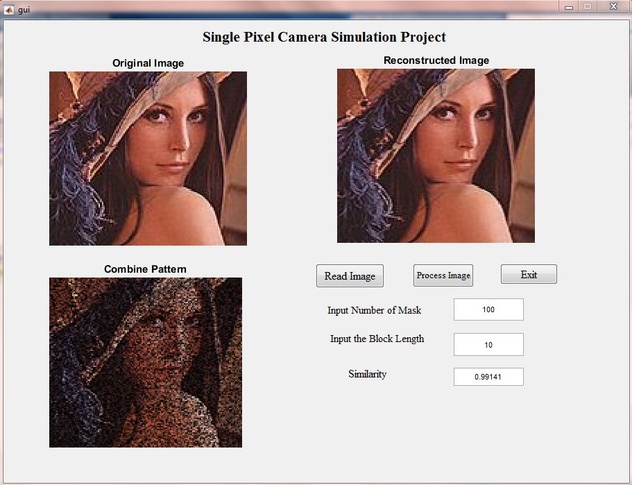
This week we tried to reconstruct a real image with different colors. The function imread() was used. The process was to reconstruct the image directly.

1.Read the image and store the data of each point in a matrix.
2.Set the numbers of the mask pattern using the numbers of pixels, this has been proved that the quality of reconstruction is the best.
3.Obtain the THz data and combine them to do the linear reconstruction. 
4.Use a simple function to compare the reconstructed image with the original image. The principle of this function is to compare the pixels of 2 different images.

We meet some problem in reconstructing the image. They are listed on the following:

1.The image should have equal length and width, the original image should be "square", the number of the pixels should be n × n.
2.MATLAB has its own limit on the size of the matrix. If the image is too large, the work can not be done. 

The flowchart is on the following: 

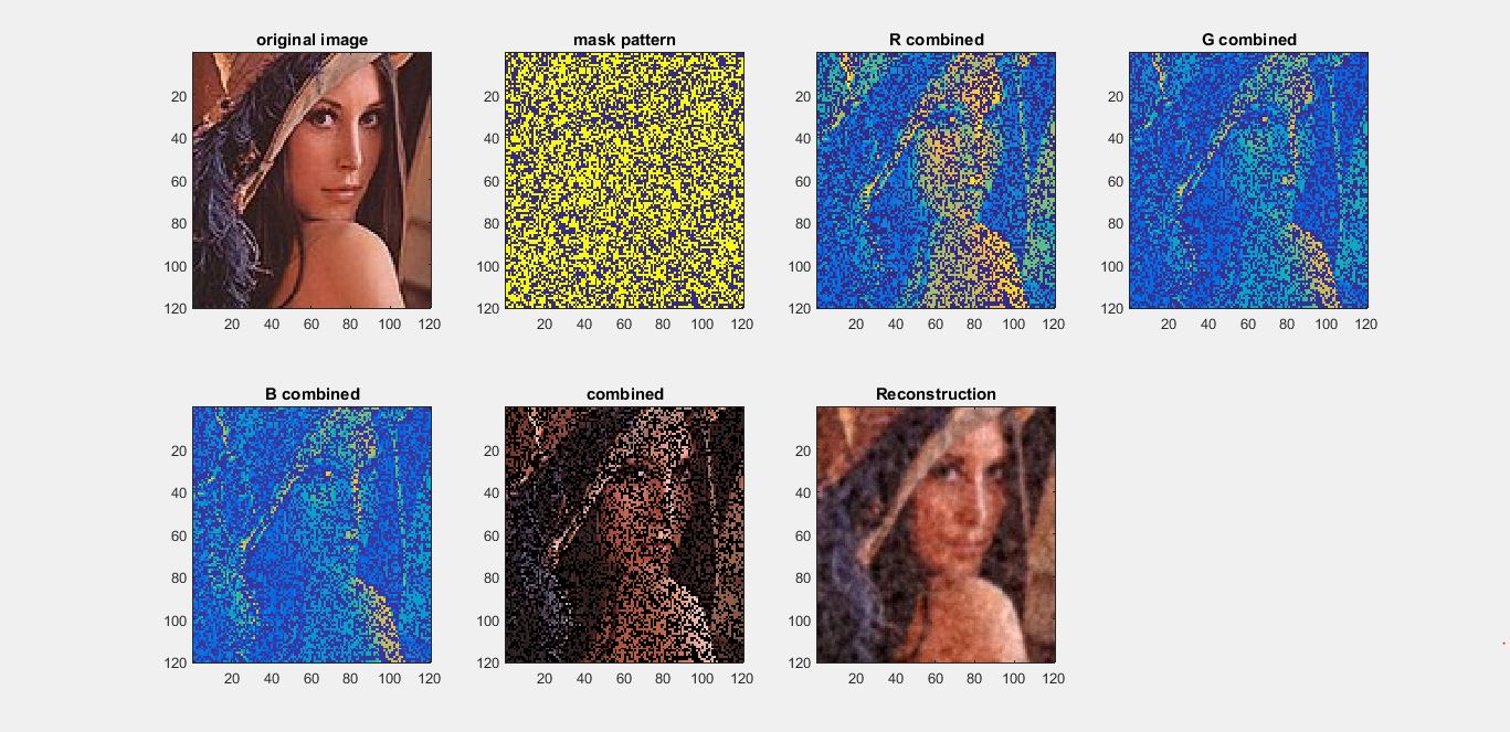
The matlab code of this part is on the following:

% test linear_rec(THzData, MaskData)

clear all;

o_ima=imread('5.jpg');

figure(1),subplot(2,3,1),imagesc(o_ima), title('original image')

% simulate mask set data

[a,b] = size(o_ima);

if a>b

   c=b;

else c=a;

end

H=im2double(o_ima);

ima=imresize(H,[c c]);

[m,n,l]=size(ima);

NP=c;

figure(1),subplot(2,4,1),imagesc(ima), title('original image')

% simulate mask set data

NM=200; % nunmber of masks

MaskData=zeros(NM,c*c);

subplot(2,4,2),im1=imagesc(ima);title('mask pattern')

subplot(2,4,3),im2=imagesc(ima);title('R combined')

subplot(2,4,4),im3=imagesc(ima);title('G combined')

subplot(2,4,5),im4=imagesc(ima);title('B combined')

for i=1:NM                                               

    temp=rand(c); temp=temp>0.5;

    MaskData(i,:)= temp(:);

    temp1=reshape(temp,c,c);%mask pattern

    set(im1,'CData',temp1);

    temp2=temp.*double(ima(:,:,1));%combined patten

    set(im2,'CData',temp2);

    temp3=temp.*double(ima(:,:,2));

    set(im3,'CData',temp3);

    temp4=temp.*double(ima(:,:,3));

    set(im4,'CData',temp4);

end

    temp5(:,:,1)=temp2;

    temp5(:,:,2)=temp3;

    temp5(:,:,3)=temp4;

    temp6=double(temp5);

    subplot(2,4,6),imagesc(temp6),title('combined');

   

    temp7=ima(:,:,1);

    THzData=double(MaskData)*double(temp7(:));

    newimg(:,:,1)=linear_rec(THzData, MaskData);

    temp7=ima(:,:,2);

    THzData=double(MaskData)*double(temp7(:));

    newimg(:,:,2)=linear_rec(THzData, MaskData);

    temp7=ima(:,:,3);

    THzData=double(MaskData)*double(temp7(:));

    newimg(:,:,3)=linear_rec(THzData, MaskData);

  

  

figure(1);subplot(2,4,7),imshow(newimg,[]);simliarity( ima, newimg );% display the reconstructed image

title('Reconstruction');

similarity(ima,newimg);

The code of the compare function is on the following:

function simliarity( ima, newimg )

%UNTITLED4 Summary of this function goes here

%   Detailed explanation goes here

I1=ima;

I2=newimg;

ssimval = ssim(I1,I2);

  

    fprintf('The ssim value is %0.4f.\n',ssimval);

  

    title(sprintf('Reconstruction - simliarity is %0.4f',ssimval));

end

And the result is on the following:

It was obviously this 2 pictures was different. The direct reconstruction illustrates failure. 

From the blog of last year, we learnt that there is one way, which was to decoration the axises with different value of the image, then combine them. Which is that we take the Red color, Green color and blue color out and to obtain the THz data, combing them separately. The flowchart is on the following:

And the matlab code:

% test linear_rec(THzData, MaskData)

clear all;

o_ima=imread('5.jpg');

figure(1),subplot(2,3,1),imagesc(o_ima), title('original image')

% simulate mask set data

[a,b] = size(o_ima);

if a>b

   c=b;

else c=a;

end

H=im2double(o_ima);

ima=imresize(H,[c c]);

[m,n,l]=size(ima);

NP=c;

figure(1),subplot(2,4,1),imagesc(ima), title('original image')

% simulate mask set data

NM=200; % nunmber of masks

MaskData=zeros(NM,c*c);

subplot(2,4,2),im1=imagesc(ima);title('mask pattern')

subplot(2,4,3),im2=imagesc(ima);title('R combined')

subplot(2,4,4),im3=imagesc(ima);title('G combined')

subplot(2,4,5),im4=imagesc(ima);title('B combined')

for i=1:NM                                               

    temp=rand(c); temp=temp>0.5;

    MaskData(i,:)= temp(:);

    temp1=reshape(temp,c,c);%mask pattern

    set(im1,'CData',temp1);

    temp2=temp.*double(ima(:,:,1));%combined patten

    set(im2,'CData',temp2);

    temp3=temp.*double(ima(:,:,2));

    set(im3,'CData',temp3);

    temp4=temp.*double(ima(:,:,3));

    set(im4,'CData',temp4);

end

    temp5(:,:,1)=temp2;

    temp5(:,:,2)=temp3;

    temp5(:,:,3)=temp4;

    temp6=double(temp5);

    subplot(2,4,6),imagesc(temp6),title('combined');

   

    temp7=ima(:,:,1);

    THzData=double(MaskData)*double(temp7(:));

    newimg(:,:,1)=linear_rec(THzData, MaskData);

    temp7=ima(:,:,2);

    THzData=double(MaskData)*double(temp7(:));

    newimg(:,:,2)=linear_rec(THzData, MaskData);

    temp7=ima(:,:,3);

    THzData=double(MaskData)*double(temp7(:));

    newimg(:,:,3)=linear_rec(THzData, MaskData);

  

  

figure(1);subplot(2,4,7),imshow(newimg,[]);simliarity( ima, newimg );% display the reconstructed image

title('Reconstruction');

similarity(ima,newimg);

In next week, we will try some other solutions to deal with large images. This week we meet the dilemma here.